
White Papers
Imaging Topics Explained
An Introduction to Digital Microscopy Imaging
As fun as taking pictures may be, it is the professional analysis of samples that really counts. This article discusses key concepts of digital imaging systems and how these concepts contribute to a professional presentation of your work.
Ensuring Maximum Resolution
The basic element of an image is the pixel. It is defined as the smallest picture element in an image. In the film medium it is the grain size of the chemicals in the film. In modern video and digital imaging cameras it is the individual, light-sensitive, silicon structure within the sensor array. The number of pixels that span the image determine the resolution of the camera. Knowing this, it can generally be said that the higher the number of pixels that span the image, the better the image quality. The ability to resolve small features with more pixels allows you to enlarge and examine these features in more detail. Maximizing the resolution in the final image is an important goal in any image system. It should be noted that each component in your imaging system has the power to degrade the resolution from theoretical maximum.
“The more pixels the better” is a generalization that has constraints. The optimum solution is one that matches the resolving power of each component in the system. Constraints on the resolution in an imaging system are the microscope objective, optical adapter, and camera. Two other important constraints are time and money.
The Microscope Objective
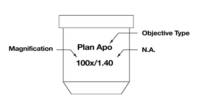
Attributes of the microscope objective that restrict resolution are the magnification – numerical aperture limit, the type of objective and the quality of manufacturing.
Magnification and numerical aperture deal with the fundamental physical principles that limit the magnification and resolution possible in light microscopy. These limits occur when each point source of light from the specimen interferes with itself causing a diffraction pattern known as an Airy Disk (a blur circle). The assembly of these blur circles at the image plane creates the image. The size of a blur circle in the image is related to the magnification and numerical aperture (NA) of the objective used (see figure #1).
The larger the NA, the smaller the blur circle. The higher the power of the objective, the larger the blur circle. If an optical system started with “zero” NA, no detail would be resolved in the image. This results from blur circles that are infinitely large, spreading their energy onto all neighboring blur circles (see figure #2).
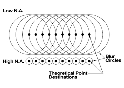
As the NA is increased for a given magnification, the resulting blur circles get smaller, concentrating more of their energy into the theoretically correct destination and contaminating less onto neighboring destinations. The image goes from “soft” with no detail, to crisp with maximum detail.
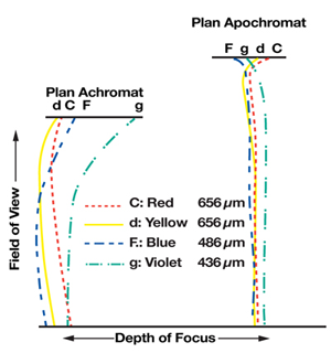
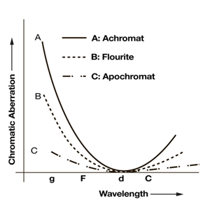
The type of objective design influences the maximum feasible NA. Each design allows different amounts of chromatic and geometric aberrations (see figures #3 and #4). For light microscopy, these designs commonly include achromat, plan achromat, plan fluorite, and plan apochromat.
Achromat designs correct chromatic aberration for 2 wavelengths of light, one in red (the C line in figure #3) and one in blue (the F line). Geometrically they are not flat field, which means the center of the field of view comes into focus at a different position than the edges. For this reason, achromat style objectives are unacceptable for image capture.
Plan Achromat designs add a correction to provide their best focus primarily in one plane. They have moderate NA and are considered the bare minimum for image capture. They are the mainstay of the industry and are moderately priced.
Plan Fluorite designs reduce aberrations further, both chromatically and geometrically. With these improvements, they are able to increase the NA for each magnification. These objectives are very strong performers and are above average in cost.
Plan Apochromat designs improve chromatic aberration correction across the entire spectrum by adding correction for the violet g line. They also achieve the highest level of geometric correction. As a result, they are designed to have the highest NA and resolving power. These objectives are astonishingly crisp in all respects. Unfortunately, this excellence comes at a much higher price than other types of objectives.
The quality of the image that the microscope sends to the camera will depend, to a great extent, on the type of objective used and on the design and manufacturing skills of its manufacturer.
The Optical Adapter
Between the microscope and the camera in the image system is the optical adapter. It can be an image quality bottleneck if it is not correctly selected. The first consideration in the selection of an adapter is whether it was designed for high-resolution cameras. Some baseline adapters optimize the cost vs. resolution balance for video systems, which have only 1/2 to 1/4 the resolution of modern digital cameras. The result could be an expensive plan apochromatic microscope objective and high-resolution digital camera crippled in resolution by an inappropriate optical adapter. Make sure that the adapter you buy is designed to handle the objective and camera you are purchasing.
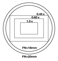
The main function of the optical adapter is to properly size the image from the microscope to fit the camera’s image sensor. The optimum magnification adapter will project a large enough image (the circular field of view from the microscope) to cover the rectangular image sensor, but not will large enlarge it to the point that only a small section of the center of the image lands on the image sensor (see figure #5). Optimal magnifications for some common image sensor formats are 0.45x – 0.55x for 1/2” CCD, 0.6x – 0.76x for 2/3” CCD, 1x for 1” CCD, 1.2x for 4/3″ CCD, 2x for digital SLR (APS-C, APS-H) sensor formats and 2.5x for full-frame (35mm) sensors. The image sensors in digital cameras don’t always conform to an industry standard format. The manufacturers of these cameras will typically provide an adapter optimized for those sensors.
Reflections within the optical system reduce contrast and color saturation. For these reasons, use of coated optics throughout the optical system is strongly suggested. Lens coatings work by reducing reflections off lens surfaces. There are two classes commonly used: single layer coatings and multiple layer coatings. Single layer coatings typically center their maximum effect in the green wavelengths. Multiple layer coatings combine three curves to more broadly cover the visible spectrum. Multi-coated lenses produce better color balance and higher contrast than uncoated or single coated lenses. Identifying the type of coating is as easy as looking at the apparent color of the lens surface. A purplish-red color indicates single coated lenses while a greenish color indicates multi-coated lenses.
The perfect optical adapter for most modern systems would be one that has no lenses and at the same time projects the appropriate field of view for the sensor used (16 – 25mm FN). This adapter would have no distortions and no photonic energy loss. The prerequisite to be able to use this type of adapter is that the sensor be of the correct size to provide appropriate field of view. Since a no-lens adapter is 1x, this corresponds to a 1” to 1.5” format sensor (16mm – 25mm diagonal).
The Sensor Array
Now that our image has made it up to the sensor plane, we can analyze the resolution needed in the camera. Knowing that NA and magnification produce a series of blur spots that make up an image, we can calculate the resolution for each microscope objective. To do this, we will normalize the image to an 18mm field of view (a conservative field number) and represent the area of interest by an inscribed rectangle (assuming proper optical adapter magnification) with an aspect ratio of 3:2. From Nyquist’s work on sampling, it is generally accepted that the blur spots should be 2 times over-sampled as a minimum requirement. This leads us to the resolutions seen in figure #6. By examining figure #6, it can be seen that at high magnification the resolution is typically constrained by the microscope optics and at low magnification the resolution is typically constrained by the camera image sensor resolution.
| Plan Achromats | Plan Flourites | Plan Apochromats | |||||||||
|---|---|---|---|---|---|---|---|---|---|---|---|
| Magnification | NA | Columns | Rows | Magnification | NA | Columns | Rows | Magnification | NA | Columns | Rows |
| 4 | 0.10 | 1364 | 909 | 4 | 0.15 | 2045 | 1364 | 4 | 0.20 | 2727 | 1818 |
| 10 | 0.25 | 1364 | 909 | 10 | 0.35 | 1909 | 1273 | 10 | 0.45 | 2455 | 1636 |
| 20 | 0.40 | 1091 | 727 | 20 | 0.55 | 1500 | 1000 | 20 | 0.75 | 2045 | 1364 |
| 40 | 0.65 | 886 | 591 | 40 | 0.85 | 1159 | 773 | 40 | 1.00 | 1364 | 909 |
| 60 | 0.80 | 727 | 485 | 60 | 0.95 | 864 | 576 | 60 | 1.40 | 1273 | 848 |
| 100 | 1.20 | 655 | 436 | 100 | 1.30 | 709 | 473 | 100 | 1.40 | 764 | 509 |
A good strategy for outfitting your imaging system (for best resolution on a limited budget) is to determine the one or two magnifications that you will commonly use for image capture. Purchase plan fluorites or plan apochromats for these magnifications along with a digital camera that does not constrain the resolution at these magnifications. Then in the future you can upgrade the other objectives and accessories.
Bit Depth
Another component of image quality is the number of brightness levels that can be represented at each pixel location. In digital imaging systems this is referred to as the bit depth. For monochrome images, the bit depth is the number of digits in the binary number for the number of brightness levels (e.g. 256 levels can be represented by 1111 1111, or 8 bits). Color image bit depths are the sum of the bit depths for each of the three primary colors (e.g. 256 levels in red, green and blue is referred to as 24 bit RGB). One bit provides two levels of brightness, black (0) and white(1). Images represented at a bit depth of one are black and white (no gray) and are hardly recognizable. Four bits provide 16 levels of brightness. Images represented with four bits would look like topographical maps since there would be bands of pixels with the same brightness levels along smoothly shaded surfaces. This phenomenon is called “banding”. Eight bits provides 256 levels of brightness, eliminating banding. 256 levels of brightness closely relates to the number of levels the human eye can discern (about 200), therefore it is used to represent gray scale images on computer monitors.
Knowing this information, it may seem that higher bit depths would be useless. In fact, twelve bits is the next level of bit depth commonly used. The value of higher bit depths comes during digital image enhancement. When image enhancement is performed, truncation of the data can occur. This phenomenon is demonstrated in the following example: If we do not use places to the right of the decimal point we would calculate “7 divided by 2” to be “3” rather than “3.5”, then multiplying “3” by “2” results in “6” rather than the “7” that we started with. In an analogous way, brightness levels can be lost during image enhancement. So if we start out with just 256 levels (8 bits) we could end up with image banding. The solution is to start out with a higher number of bits.
Hardware Considerations for Achieving High Bit Depth
Since high bit depth is desirable, how do manufacturers achieve it? High bit depth resolutions are achieved by increasing the signal to noise ratio in the analog part of the system and then digitizing the signal with 14-bit analog to digital converters. Scientific grade CCD sensors are the first step in increasing the signal quality. These sensors have larger pixel wells that provide a greater dynamic range. In addition these CCD sensors have less variation between pixels and are individually graded for this characteristic. Consumer grade sensors reduce silicon real estate to save money while accepting higher defect and pixel to pixel variation. To further reduce noise, 14-bit camera manufacturers cool the imaging sensors. This halves the sensor noise for every 5-7° C of cooling. Temperature differentials of -10° C to –40 °C from ambient air temperature are typical cooling specifications. Cold image sensors allow you to take images of dim specimens without the image being overwhelmed by noise. Another feature that reduces noise is performing 14-bit sampling of each pixel as close to the image sensor as possible. This avoids long printed circuit board traces and cables that can act as antennae picking up electromagnetic noise from the surrounding environment. Contrast this scenario with video grabber systems that first create a video signal then send it out long cables to be decoded and digitized.
Color Representation
To understand color it is helpful to understand how the human eye perceives color. The eye has three types of color sensors, one each for “red”, “green” and “blue” light. In actuality the “red” sensor is sensitive to the color spectrum from deep red to deep green, the “green” sensor is sensitive to the color spectrum from deep orange to deep turquoise, and the “blue” sensor is sensitive to the color spectrum from deep green to deep violet. Because of this arrangement, the brain receives only three brightness inputs from each eye “pixel” to represent all perceived colors. This is why there are three primary emissive colors, red, green and blue. These differ from the primary absorptive colors of red, yellow and blue, in that the emissive colors are additive (red, green and blue light add to make white light) were as the absorptive colors are subtractive (red, yellow and blue dye add to make black).
The other characteristics of these primary colors are similar to what you learned in grade school. By mixing primary colors we can represent any other color. The color produced is related to the ration (brightness) of each primary color contributed to the mix. As with the monochrome case, each eye sensor type has sensitivity of about 256 levels of red, green or blue brightness.
Knowing this information, digital color image representation was designed to:
- Measure the brightness of light within each primary color spectrum;
- Present this data to the eye either through absorptive representation (photos and prints) or through emissive representation (CCTV or computer monitors);
- Have a digital standard for final output of data to the eye of 256 levels of brightness per primary color, (8 bits-red) + (8 bits-green) + (8 bits-blue)= (24 bit RGB color);
- Should have image capture at a higher bit depth to avoid truncation errors and banding, (14 bits-red) + (14 bits-green) + (14 bits-blue)= (42 bit RGB color).
Capturing Color
Splitting the digital color data results in images of red, green and blue intensities. These images are called “color planes”. CCD and CMOS sensors are inherently “black and white”. They require the addition of color separation filters to capture each of the color planes needed to create the color image. Several different techniques are used to create color images.
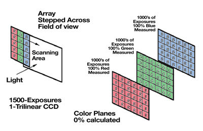
Three-Color Scanning Technique
This technique employs an array that is made up of three columns. Each column is dedicated to one of the primary colors. The array is stepped across the image perpendicular to the three columns. At each step, the array is read out capturing the red, green and blue data at each pixel location (see figure #7). The advantage of this type of camera is the reduction of sensor cost while achieving non-interpolated, high-resolution images. The disadvantages of this system are image acquisition time (1 to 2 minutes), possible image blur due to step vibration, light source variation during image capture causing brightness variation between columns and the inability to capture images of moving specimens.
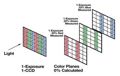
Color Mosaic Sensor Technique
This technique applies a mosaic of color filters directly onto the silicon sensor during the manufacturing process. The filters are most commonly applied in a repeating, four-pixel element called a Bayer Filter Pattern. Individual pixels then acquire red, green, or blue light intensity with the missing two color values interpolated from neighboring pixels. This method has the advantage of low cost and ability to capture moving specimens without color ghosting. The time to capture and display the image is equal to the time to expose and down load one frame plus the time to interpolate the missing colors. The disadvantage is the loss of resolution. The resolution in each color plane is only 25% to 50% of the sensor resolution depending on the mosaic pattern. With 67% of the image data being calculated, an additional problem is interpolation artifacts and distortions. Black lines appear as striped lines and edge details become distorted and “blocky” (see figure #8).
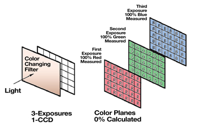
Three-Shot Single Sensor Technique
Three-shot single sensor cameras place a filter assembly in the front of the camera and sequentially expose the sensor to each of the three primary colors.
This method solves the interpolation problem by providing 100% measured data for all color planes. The time to capture and display the image is equal to the time to expose and download three frames. The prices are comparable or slightly more expensive than color mosaic cameras while providing 2 to 3 times higher resolution. The disadvantage is on capturing moving specimens. Since the images are taken sequentially, a moving specimen will be in a different position during each color exposure. The composite image of a moving specimen would then show three “color ghosts” of the item that moved.
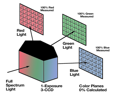
Single-Shot Three Sensor Technique
Three sensor cameras seek to solve the interpolation problem by splitting the light into its three color bands with prisms and dichroic filters. Each color band is sent to its own dedicated image sensor and circuit. The time to capture and display the image is equal to the time to expose one frame and download three frames of data. The advantage here is measurement of every color at every pixel location. Additionally, since the images are captured simultaneously, moving specimens do not have color ghosting problems. The disadvantage is that this camera has three times the cost in sensors and circuitry as well as in the complex optical element. The result is high prices and is an expensive solution if your specimen is not moving (see figure # 10).
Mechanical vs. Electronic Shuttering
A final subject to cover in this article is shuttering. Shuttering is the operation of starting and stopping the collection of light on the image sensor. There are several different types of sensor architecture. For sensors using the full-frame architecture, the pixels in these devices are continuously sensitive to incoming light. They require an external shutter to block the light before and after the exposure. Another type of image sensor architecture is called interline. Interline image sensors have an electronic storage area between each pixel column which acts as an electronic shutter and enables the sensor to protect the pixel data from exposure during readout. The elimination of the mechanical shutter has several advantages. First, electronic shuttering can accommodate exposures 80 times shorter (brighter) than mechanical shutters. Next, this high speed shuttering makes real time viewing possible, giving digital cameras many of the user-friendly features of video cameras. Finally, since there are no moving parts, there is no wear or mechanical failure of the shutter, which is the highest maintenance component in full-frame cameras.